
Return of the Multiple
Return of the Multiple
Manager Selection and Capital Allocation
Part 2 of this series on measuring returns looks at multiples or ‘times capital returned.’
In part 1, I explained that while IRR is useful, it has limitations. That there is a trade-off when using one tool over another and no metric should be used in isolation.
Let’s use the example from the last article to illustrate. Now there is an extra $10 distribution in year 3 for Option B; this equalises IRR for both options. Option B now looks even more attractive, with $60 profit as opposed to $25 for Option A. However, looking at the IRR only, we’d conclude both options are equally as good at 22% p.a.
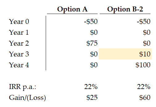
This problem is particularly evident when comparing returns of a buyout fund with a venture fund. We can expect a buyout fund will return capital to investors quicker than a venture fund. Generally, buyout funds pull shorter-term levers to realise value (paying off debt, improving profitability, buying low/selling high). On the other hand, venture funds must support nascent businesses over the longer haul to realise a home run (or not). For simplicity, we’ll assume Option A is a buyout fund and Option B is a venture fund.
There’s a quick and easy way to compare these two seemingly equal options: a multiple or ‘times capital returned.’ For Option A the multiple is $75 on capital of $50 = 1.5x. For Option B-2, the multiple is $110 on capital of $50 = 2.2x. Easy.
These multiples apply to the private equity fund, not the underlying investment. Option A is not saying $50 was invested into a company and that company is now worth $75; it is saying that $50 was contributed (or ‘paid-in’) to the fund by the investor (e.g. funding investments, management fees and expenses) and then $75 cash was distributed to the fund back to the investor. These are net returns to investors after fees.
We now see why it’s important not to rely solely on IRR. Using the buyout versus venture example, we know that venture must have a higher multiple target than buyout to achieve the same IRR.
Distributions to Paid-In Capital (DPI)
More formally, the multiple above is ‘Distributions to Paid-in Capital’ or ‘DPI’. This is cash returned to the investor divided by cash contributed by the investor.
Paid-in to Committed Capital (PICC)
As I wrote in Alpha Allocators, committed capital is not the amount of capital put to work. If an investor commits $10m, then that $10m won’t be invested immediately but contributed (paid-in) over time. For argument’s sake, let’s say our investor has committed $200 to the fund. A metric that shows how much capital has been paid-in versus total committed is ‘Paid-in to Committed Capital’ or ‘PICC’:

Residual Value to Paid-in Capital (RVPI)
Going back to our cashflow diagram for private equity:

There are two components of the value to investors. While distributed capital is the cash returned to investors, there’s also a residual value in the remaining investments (e.g. companies yet to reach a liquidity event). One way to think of this residual value or ‘Net Asset Value’ is the gain or loss on paid-in capital, less distributions already made to investors:

To quantify residual value on relative terms, we use ‘Residual Value (or Net Asset Value) over Paid-in Capital’ or ‘RVPI’. Let’s say the fund in Option A has valued its investments at $50:
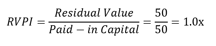
Like the other metrics, RVPI is a net return, so the numerator is after fees, carried interest and expenses (as is the Gain/(Loss) in the NAV equation above).
Total Value to Paid-in Capital (TVPI)
Putting distributed value and residual value together, we get the most useful net multiple metric: ‘Total Value to Paid-in Capital’ or ‘TVPI’. Useful because neither distributed capital or residual value by themselves tell the full story; they are interim measures. There may be more distributions to come and the value of those distributions is the residual value. Our TVPI would be:

Total Value to Committed Capital (TVCC)
The multiples above do not account for capital yet to the contributed (paid-in) by the investor, sometimes referred to as ‘undrawn capital’. Remember, the investor commits a certain amount, but this commitment is only drawn over time; the capital ‘in the ground’ at any one time will never reach this commitment. Using the multiples above, we can draw only conclusions on the returns earned on paid-in capital and not total committed.
A seldom-used multiple that accounts for undrawn capital is ‘Total Value to Committed Capital’ or ‘TVCC’. For simplicity, say the investor committed $50 to Option A above. Then, TVCC=TVPI and everything is golden. However, if the investor committed $200, then TVCC is:

In the early years, 0.625x TVCC might be fine. However in year 10, if TVPI = 2.5x and TVCC = 0.625x then something has gone wrong. Why did the fund stopped calling capital from investors and stop making investments? If you commit a certain amount, you’d want the fund to call close to that amount.
Like every metric in private equity, the vintage of the fund should be read alongside TVCC. TVCC will only become useful as we travel along the J-curve in subsequent years. Rather than an absolute performance metric, I like to use TVCC to compare funds of the same strategy and same vintage; I can then get a feel for how much capital was paid-in and put to work out of the total commitment.
Multiple Nuances
There are some nuances and drawbacks when using multiples :
Multiples tell you nothing about time - a 2x return is good over 4 years but not so good over 15. In one sense, this is not a big issue provided the investor accepts that private equity is a long term investment and a range of metrics are used together.
While TVPI is the most relevant metric for overall performance, it is not the most reliable - the residual value component is an estimated valuation by the fund (according to its policy). Valuation is subjective. I have yet to see any firm, advisor or auditor with the same valuation approach. Every quarter is an exercise in establishing a common language between the valuer and auditor (at least at first). Some organisations have made efforts to provide consistent guidelines, and some of these are very good, but adoption varies.
The multiples in this article are net multiples, which are useful to evaluate overall returns but not as useful evaluating the raw investing acumen of the fund and team. For example, a low TVPI may be dragged down by fees and belies great investments on a gross basis (the right side of the cash flow diagram above). The investor needs to work out if a lower net multiple is a result of poor investments returns (any why), excessive fee drag or both.
Conclusion
Multiples are an easy and useful metric that should be used alongside IRR to provide a more fulsome picture of fund return and performance.
To calculate these multiples, all you need are the series of cash flows over time or the aggregate amounts for each of Paid-in Capital, Distributions and NAV (and Committed Capital to work out TVCC). If you’re using the fund cash flows, the negative cash flows are paid-in capital, the positive are distributions and the final cash flow line item is usually the NAV, if not split out separately. (In practice, this might not always be true, e.g. there might be positive/negative adjustments for revaluations).

Assessing fund performance is difficult. Using qualitative in addition to quantitative factors is not a platitude, it is a necessity as we can see from the discussion on performance metrics so far. No single number can ever provide the full picture and can lead to poor investment decisions or missed opportunities. The more inefficient the asset class, the more important qualitative factors become.